The law of variable proportion occupies an important place in economic theory. This law examines the production function with one factor variable, keeping the quantities of other factors fixed. In other words, it refers to the input-output relation when output is increased by varying the quantity of one input. When the quantity of one factor is varied, keeping the quantity of other facts constant, the proportion between the variable factor and the fixed factor is altered; the ratio of the variable factor to that of the fixed factor goes on increasing as the quantity of the variable factor is increased. Since under this law we study the effects on output of variation in factor proportions, this is known as the law of variable proportions. Thus law of variable proportions the new name for the famous “The Law of Diminishing Returns” of classical economics. This law has played a vital role in the history of economic thought and occupies an equally important place in modern economic theory. This law has been supported by the empirical evidence about the real world. The law of variable proportions or diminishing returns has been stated by various economists in the following manner:
“As the proportion of one factor in a combination of factors is increased, after a point, first the marginal and then the average product of that factor will diminish.” (F.Benham)
“An increase in some inputs relative to other fixed inputs will, in a given state of technology, cause output to increase; but after a point the extra output resulting from the same addition of extra inputs will become less.” (Paul A. Samuelson)
Marshall discussed the law of diminishing returns in relation to agriculture. He defines the law as follows: “An increase in the capital and labour applied in the cultivation of land causes, in general, a less than proportionate increase in the amount of product raised unless it happens to coincide with an improvement in the arts of agriculture.”
It is obvious from the above definitions of the law of variable proportions that it refers to the behaviour of output as the quantity of one factor is increased, keeping the quantity of other factors fixed and further it states that the marginal product and average product will eventually decline.
Assumptions of Law of Variable Proportion
The law of variable proportion holds good under the following assumptions:
1. The state of technology is assumed to be constant. So there could be no improvement in technology in between when we are analysing the production function using this law. Because if improvement in technology is permitted then marginal and average product may rise given same level of inputs on account of better available technology.
2. Only one factor at a time assumed to be variable and all other factors are assumed to be fixed because then only we can study that what would be the change in output due to change in variable factor.
3. Different units of variable factors are assumed to be homogeneous. Because if they are not homogeneous then we can’t study the impact of change in variable factor only, then production function will show combined effect of change in variable input simultaneously with quality of input. (Heterogeneous inputs imply different quality).
4. The law is based upon the possibility of varying the proportions in which the various factors can be combined to produce a product. The law can’t be applied to those cases where the factors must be used in fixed proportions to yield a product. The law as formulated by Joan Robinson is widely used law of production in short-run analysis. The law states that as a producer employee successive units of variable factor with given amount of fixed factors, then initially marginal productivity will increase, followed by a decrease and ultimately will become negative.
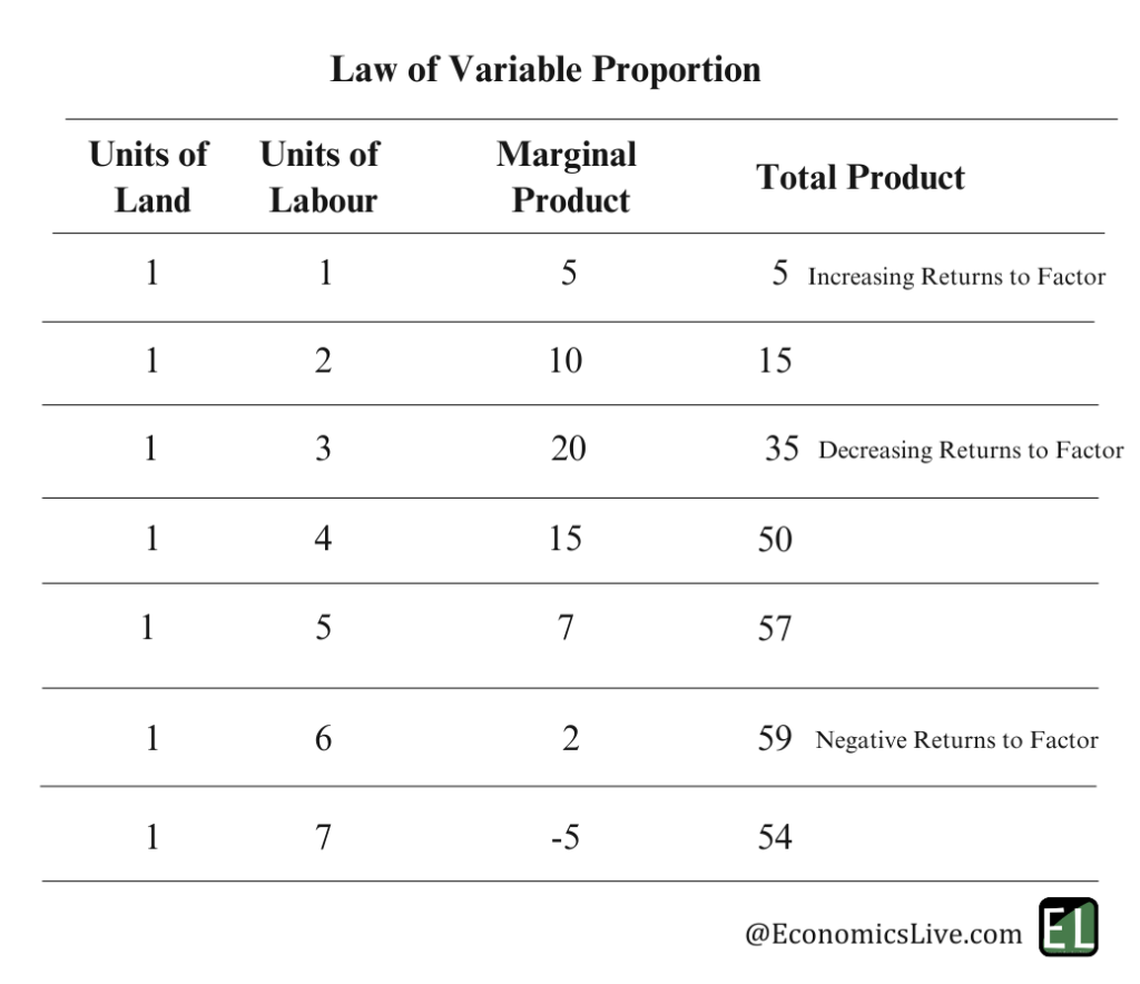
In other words as a producer combines additional units of a variable factor with given amount of fixed factors, the total product increases, but after a point of time starts falling. We shall explain this law using a schedule and diagram. We assume that there is a fixed amount of land available for production and labour is the only variable factor.

So, we see that as producer kept on increasing the labour inputs, initially till 3rd labour input marginal product increased, then after 3rd unit it started declining and became negative after 6th unit of labour, leading to negative returns to factor.
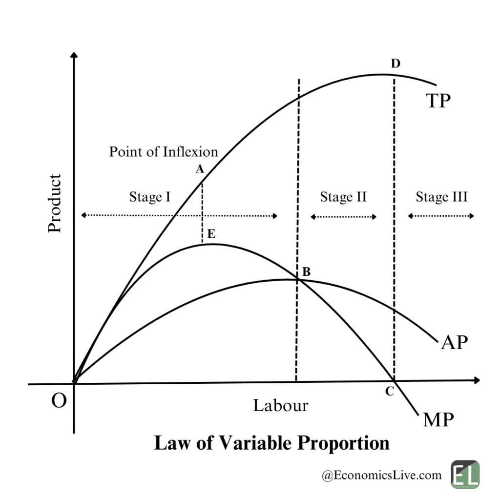
When MP increases, then TP TP increases at increasing rate and as MP falls, TP still increases, but at a decreasing rate and as MP becomes negative, TP starts falling.

In the above diagram as we can see as a Labour inputs increases on x-axis, the MP of labour increases, till point E and in corresponding to it TP increases at increasing rate till point A. After point A TP increases at decreasing rate. After point A TP increases at decreasing rate. So, point A is also called as point of inflexion, because the TP curve changes its curvature at point A.
At point B, average product is maximum which means AP=MP, at point B, which marks the end of first phase of production which is otherwise known as phase of increasing return.
In Stage II MP is continuously falling and TP is increasing at a decreasing rate and finally touches x-axis at point C, where MP=0 and TP is maximum at corresponding point D. From point C onwards phase III sets in which is called the phase of negative returns.
A national producer will always operate in stage II of production. Stage III is ruled out because 7 gives negative returns and in phase I MP is rising and later begins to fall, which means addition to TP. On first phase a producer will not stop because fixed factors of production have not been fully used unto their potential.
Thus, a rational entrepreneur will not stop in phase I and will expand his production till marginal product become zero, which means till MP=0, hiring an extra variable input was contributing something to the TP.
So it it clear that producer will not operate in either stage I or stage III. Therefore stage I and stage III are called as stage of economic absurdity or economic non-sense. So, stages I and III represent non-economic regions in production function.
Causes of Increasing Returns
In beginning the quantity of fixed factor of production is abundant relative to the quantity of the variable factor. So, when more variable factor is added then efficiency of fixed factor increases.
The second reason is that as more units of the variable factors are employed the efficiency of the variable factor itself increases. This is because when there is sufficient quantity of the variable factor, it becomes possible to introduce specialisation or division of Labour which results in higher productivity.
Causes of Diminishing Returns
Once a point is reached at which the amount of variable factor is sufficient to ensure the efficient utilisation s of fixed factors, then any further increase in variable factor will lead to fall in marginal and average products, because fixed factor become inadequate in relations to variable factors.
Mrs Joan Robinson further said that we get diminishing returns because factor of productions are not perfect substitutes for each other. So, after a point need for more fixed factors can’t be substituted by increasing variable factors of production
So, diminishing returns operates because the elasticity of substitution between factors is not infinite.