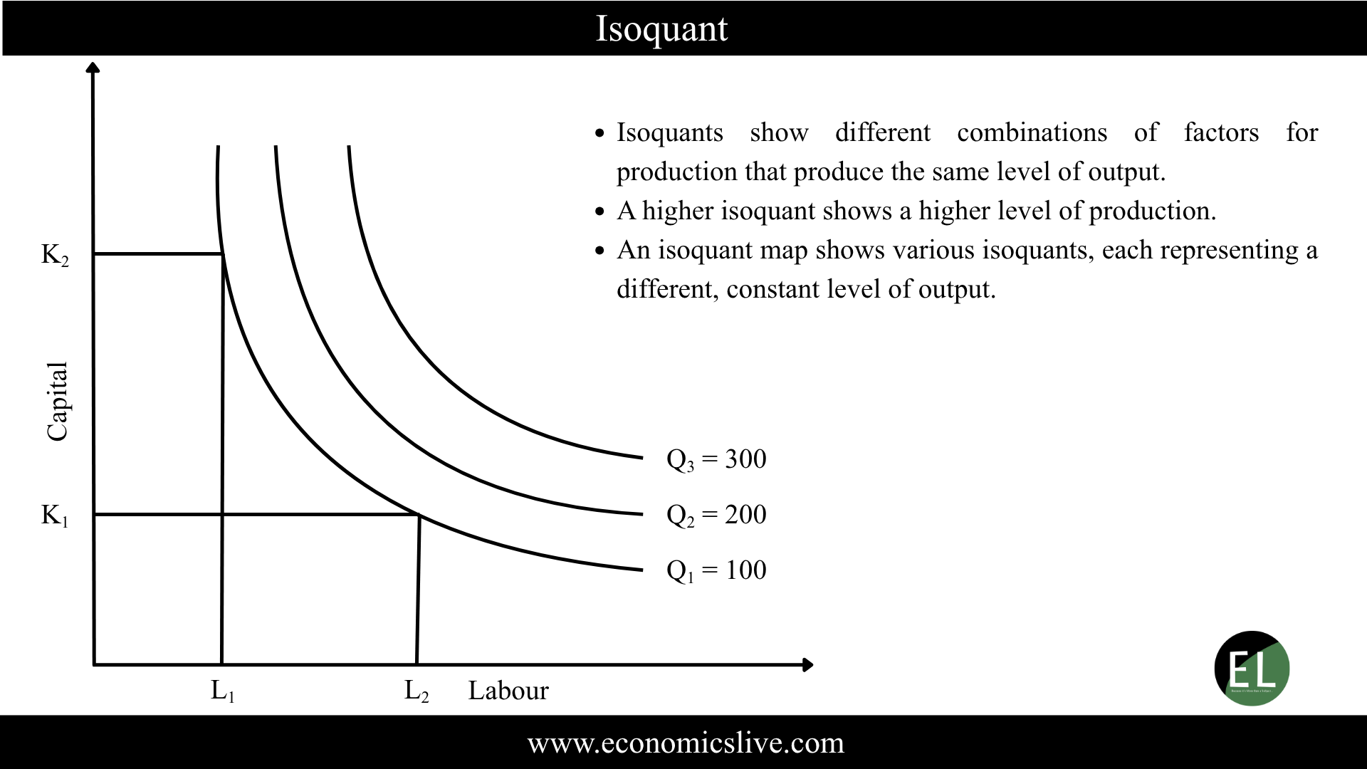
An isoquant (also known as an Equal Product Curve) is a curve that shows all possible combinations of two inputs, such as labor (L) and capital (K), that produce the same level of output. In simple terms, it represents different input combinations that yield an identical quantity of production.
The term Isoquant is derived from two Greek words:
- “Iso” meaning equal, and
- “Quant” meaning quantity.
Hence, an isoquant literally means equal quantity.
Mathematically, if the production function is expressed as \(Q=f(L,K)\) then, for a given level of output \(Q_0\), the isoquant represents all combinations of \(L\) and \(K\) that satisfy: \(f(L,K)=Q_0\).
Each isoquant corresponds to a specific level of output and higher isoquants denote higher levels of production. In simple words, an isoquant is a producer’s tool to identify how labor and capital can be adjusted against one another while keeping output unchanged.
It can be illustrated with the help of following table:
| Factor Combination | Labor (L) | Capital (K) |
| A | 10 | 5 |
| B | 7 | 8 |
| C | 5 | 10 |
Suppose a factory produces 100 units of a commodity. These can be produced using the various combinations mentioned above. For example, 100 units of a commodity can be produced with combination A, which comprises 10 units of labor and 5 units of capital. Alternatively, another combination, B, comprises 7 units of labor and 8 units of capital. They can be produced using A, B, or C, and all combinations yield the same level of production. It can be shown with the help of following diagram:

Mathematical Expression of Isoquant
Consider the Cobb-Dauglas production function, which is a common representation in production theory:
\(Q=AL^{\alpha}K^{\beta}\)Where:
\(Q=\)Output
\(L=\)Labour input
\(K=\)Capital input
\(A=\)Total factor productivity (Technology constant)
\(\alpha, \beta = \) Output elasticities of labour and capital respectively
For a given level of output \(Q_{0}\), we can derive the isoquant as:
\(K=\left(\frac{Q_0}{AL^\alpha}\right)^{1/\beta}\)This mathematical form shows all combinations of labour and capital that maintain the same output level \(Q_{0}\).
Properties of isoquants
1. Isoquants slope Downwards from left to Right
The isoquant is negatively sloped, which means that it moves downward from left to right.
This property reflects the substitution effect between inputs: to maintain the same output, an increase in one input say labour, must offset by a decrease in the other i.e., capital. If labour increases, capital must decrease, keeping the total production constant.
Mathematically,
\(\frac{\partial L}{\partial K} < 0\)This negative slope demonstrates that both inputs contribute positively to production and can substitute for each other to a certain extent.
2. Isoquants are convex to the Origin
The convex shape of an isoquant arises because of the Law of Diminishing Marginal Rate of Technical Substitution (MRTS).
The MRTS measures how much of one input (e.g., capital) must be reduced when one more unit of another input (e.g., labor) is added, keeping the output constant.
\(MRTS_{LK} = – \frac{\partial L}{\partial K} \)As more labor is used in place of capital, the producer can afford to give up less capital for each additional unit of labor. This diminishing substitution effect results in a convex isoquant.
If isoquants are concave, it violates the principle of diminishing returns, which seldom occurs in real production systems.
3. Higher isoquants represent higher levels of output
Isoquants located farther from the origin indicate higher output levels as they represent greater combinations of inputs.
For instance:
\(Q_{1}=\) 100 units of output
\(Q_{2}=\) 100 units of output
\(Q_{3}=\) 100 units of output
Thus, each higher isoquant reflects an increase in the total product, assuming positive marginal productivity of inputs.
4. Isoquants Never Intersect Each Other
The two isoquants cannot intersect because this implies that a single input combination produces two different levels of output, which is logically impossible.
Each isoquant represents a unique quantity of output, which ensures the consistency of the production function.
5. Isoquants Do Not Touch the Axes
An isoquant never touches the X or Y – axis because no output can be produced using only one input.
In the long run, both labor and capital are essential for production. Thus, points on either axis where one input is zero are technically infeasible.
6. The shape Depends on the Degree of Substitutability Between Inputs
The curvature of an isoquant reflects how easily one input can be substituted for another:
| Type of Input Relationship | Substitutability | Shape of Isoquant |
|---|---|---|
| Perfect Substitutes | Complete substitutability | Straight line |
| Perfect Complements | No substitutability (fixed proportions) | Right-angled (L-shaped) |
| Imperfect Substitutes | Partial substitutability (real-world case) | Smooth, convex curve |
Types of Isoquants
Isoquants vary according to the technological relationships between inputs. Following are the three common types of isoquants:
1. Linear Isoquant (Perfect Substitutes)
When labor and capital can completely replace each other at a constant rate, the isoquant is linear.
Example:
\(Q = \alpha L + \beta K\)Here, one unit of capital can always substitute for a specific number of labor units, and vice versa.
Such cases are rare in real life but can be found in industries where automation and human labor can be perfectly substituted (e.g., self-checkout vs cashier).
2. Right – Angled Isoquant (Perfect Complements)
When production requires inputs in fixed proportions, the isoquant takes the right-angled (L-shaped) form.
Example:
\(Q=\min(aL,bK)\)In such cases, increasing one input while holding the other constant does not increase output.
For example, if one machine requires one operator, having extra machines without additional workers (or vice versa) will not increase production.
3. Smooth Convex Isoquant (Imperfect Substitutes)
Most real-world production systems exhibit imperfect substitutability between the inputs.
Here, the isoquant is smooth and convex to its origin, reflecting a diminishing MRTS.
Example:
\(Q = A L^{\alpha} K^{\beta}\)
Such isoquants represent the Cobb–Douglas production function, which is widely used in empirical economic research.